R and Quakes
Update: The 6.0 Napa earthquake occured a week after I originally published this post. I re-ran the code and analysis to include the latest activity.
I decided to do a bit of data exploration around major California earthquakes in the last 30 years. Specifically, I will look at earthquakes within 200 km of San Francisco and Los Angeles between August 1984 and August 2014.
USGS has a very accessible Earthquake API and online query form. I wrote a simple script in Python3 which queries the API and downloads the result.
Data preparation
Fetching the data
To pull down the data, use usgs.APIquery with the desired parameters. All parameters are defined here.
import usgs

# obtain data for the greater San Francisco area, start of 1984 through August 24, 2014 in PST
usgs.APIquery(starttime = "1984-01-01T07:00:00", endtime = "2014-08-25T07:00:00",
              minmagnitude = "1.5",
              latitude = "37.77", longitude = "-122.44",
              minradiuskm = "0", maxradiuskm = "200",
              reviewstatus = "reviewed",
              filename = "usgsQuery_SF_84-14.csv",
              format = "csv")

# obtain data for the greater Los Angeles area, start of 1984 through August 24, 2014 in PST
usgs.APIquery(starttime = "1984-01-01T07:00:00", endtime = "2014-08-25T07:00:00",
              minmagnitude = "1.5",
              latitude = "34.05", longitude = "-118.26",
              minradiuskm = "0", maxradiuskm = "200",
              reviewstatus = "reviewed",
              filename = "usgsQuery_LA_84-14.csv",
              format = "csv")
Switching over to use R, I then read the CSVs into dataframes. For convenience, I define an area label and combine the dataframes into one.
SFquakes = read.csv("usgsQuery_SF_84-14.csv", header = TRUE, stringsAsFactors = FALSE)
LAquakes = read.csv("usgsQuery_LA_84-14.csv", header = TRUE, stringsAsFactors = FALSE)
SFquakes$area = "SF"
LAquakes$area = "LA"
quakes = rbind(SFquakes, LAquakes)
Data scrubbing and binning
# remove columns with all NA values
quakes = quakes[,-7:-10]

# create column with time object
quakes$ptime = as.POSIXlt(strptime(quakes$time, "%Y-%m-%dT%T"))

# remove instances of mwb, an alternative form of magnitude measurement
quakes = quakes[-which(quakes$magType == "mwb"),]

# create columns with year bins
quakes$yearbins = strftime(cut(quakes$ptime, "year", right = F), "%Y")

# keep one significant figure after the decimal point for magnitude
quakes$mag = round(quakes$mag, 1)

# create columns with half and whole magnitude bins
quakes$Mhalfbins = cut(quakes$mag, seq(2.0,7.5,.5), right = F)
quakes$Mwholebins = cut(quakes$mag, seq(2.0,8.0,1), right = F)

# create a column with varied magnitude bins, necessary if plotting without a log scale
quakes$Mvariedbins = cut(quakes$mag, c(2.0,2.5,3.0,3.5,4.0,5.0,7.5), right = F)
Magnitude-energy conversion
One way to comprehend the destructive force of earthquakes is to convert from earthquake magnitude to a more imaginative unit of energy: the ton of TNT. To do this conversion, we need to be able to convert from magnitude to energy, perhaps with the help of Beno and Charles. Also, it is useful to know that one ton of TNT is equivalent to about 4.184e9 Joules.
The Gutenberg and Richter energy-magnitude relation (in Joules):
E[M] = 10^(1.5M + 4.8)
quakes$Ejoules = 10^(1.5*quakes$mag + 4.8) # units of Joules
quakes$Etnt = quakes$Ejoules/4.184e9       # units of kilotonnes, TNT
Calculate approximate distance from epicenter to city center
For this calculation I decided to use the Haversine formula. A great reference to implementing this method and other methods can be found here.
Rearth = 6371 # average earth radius

# approximate city centroids
quakes$area_lon = 0
quakes$area_lon[quakes$area == "SF"] = -122.44
quakes$area_lon[quakes$area == "LA"] = -118.26
quakes$area_lat = 0
quakes$area_lat[quakes$area == "SF"] = 37.77
quakes$area_lat[quakes$area == "LA"] = 34.05

# haversine formula
lat1 = quakes$area_lat*pi/180
lat2 = quakes$latitude*pi/180
dlat = (quakes$area_lat - quakes$latitude)*pi/180
dlon = (quakes$area_lon - quakes$longitude)*pi/180
a = sin(dlat/2)*sin(dlat/2) + cos(lat1)*cos(lat2)*sin(dlon/2)*sin(dlon/2)
c = 2*atan2(sqrt(a), sqrt(1 - a))
quakes$dist = Rearth*c
Ask the data
What were the largest earthquakes in recent history?
quakes = quakes[order(quakes$mag, decreasing = TRUE),] # sort by magnitude
print(quakes[quakes$mag >= 6.0,c("ptime", "mag", "area", "Etnt", "dist")])
Output (with annotation):
                    ptime mag area       Etnt      dist
15826 1992-06-28 11:57:38 7.3   LA 1344028.02 159.76987 <-- Landers
12577 1999-10-16 09:46:46 7.2   LA  951498.97 175.46360 <-- Hector Mine
6365  1989-10-18 00:04:16 6.9   SF  337604.58  94.25933 <-- Loma Prieta
14411 1994-01-17 12:30:55 6.7   LA  169203.10  31.30647 <-- Northridge
15814 1992-06-28 15:05:33 6.5   LA   84802.44 135.38916 <-- related to Landers
7197  1984-04-24 21:15:20 6.1   SF   21301.41  82.69884 <-- Morgan Hill
16096 1992-04-23 04:50:23 6.1   LA   21301.41 162.05213 <-- Joshua Tree, preceeded Landers
6     2014-08-24 10:20:44 6.0   SF   15080.24  51.28585 <-- Napa
To compare the largest earthquakes in each area, the Landers quake had an explosive force of 1.3 megatonnes of TNT, while the Loma Prieta had about 340 kilotonnes of explosive force.
Since epicenter location is a huge factor in the destructive power of an earthquake, it is interesting to note that the Landers quake was about 160 km away from the densely populated LA metro area, while the Northridge quake was 30 km away, and about 4.0 (10^.6) times less powerful.
Which major city was most affected by earthquakes?
# Mean distance, magnitude, and Energy in TNT
print(aggregate(data = quakes, cbind(dist, mag, Etnt) ~ area, mean))
Output:
  area     dist      mag      Etnt
1   LA 124.8353 2.796353 273.54752
2   SF 115.9873 2.589565  56.07969
The question of which city has been more affected is more complex than a simple calculation of the 30-year mean of distance and magnitude. However, on average, recent earthquakes surrounding LA have been about 10% closer than Bay Area earthquakes, 1.6 (10^.21) times more severe in magnitude, and with over 4 times more explosive force.
What is the combined yearly mean distance, magnitude, and energy?
# yearly averages
print(aggregate(data = quakes, cbind(dist, mag, Etnt) ~ yearbins, mean))
Output:
yearbins      dist      mag         Etnt
1      1984 109.04522 3.351741  118.2368472
2      1985 119.81664 3.106047    7.7798894
3      1986 123.08929 3.196345   57.9139893
4      1987  97.24530 3.098084   28.2857204
5      1988 117.30689 3.134848   14.5052295
6      1989  99.45154 3.223005  804.5486309
7      1990 109.68262 3.072021   23.2815528
8      1991 113.49903 3.020319   24.0027741
9      1992 156.32608 3.237759  983.2753462
10     1993 135.49608 2.986907    2.7064472
11     1994  70.18247 3.157971  168.1940170
12     1995 138.14896 3.124582   17.2462753
13     1996 129.99745 3.138735    6.0027307
14     1997 115.75065 3.156890    6.6688196
15     1998 117.41048 3.114228    6.7265345
16     1999 172.62893 3.256908 1310.8670301
17     2000 149.68578 3.105828    4.8142657
18     2001 137.13644 3.147203    7.0122122
19     2002 117.39979 3.076856    4.3661773
20     2003 121.76297 3.115162    6.3490834
21     2004 119.03760 3.097368    8.9307051
22     2005 121.67829 3.138785   13.8969863
23     2006 121.59305 3.050495    3.9256528
24     2007 114.70162 3.046964   19.8885765
25     2008 113.91730 2.963265   12.9691261
26     2009  96.35781 2.678468    3.1106334
27     2010 104.13835 2.665835    1.2364846
28     2011  99.73551 2.676221    1.5248688
29     2012 104.98631 2.606157    1.1377617
30     2013 125.22960 1.933424    0.3044841
31     2014 118.96839 1.942429    6.8136214
Due to the exponential nature of the data, the Etnt feature is a clear indicator for seismologically active years. Also, it appears we are seeing increased detection efficiency in the last few years with the average magnitude decreasing. Note, however, that 2014 is not a complete year at the time of this blog post.
What is the magnitude-frequency distribution for the two areas of interest?
freqSF = as.data.frame(table(quakes[quakes$area == "SF","Mhalfbins"]))
names(freqSF) = c("magSF", "freqSF")
freqLA = as.data.frame(table(quakes[quakes$area == "LA","Mhalfbins"]))
names(freqLA) = c("magLA", "freqLA")

# event frequency
print(cbind(freqSF, freqLA))
Output:
     magSF freqSF   magLA freqLA
1  [2,2.5)   1215 [2,2.5)   1018
2  [2.5,3)   2069 [2.5,3)   2600
3  [3,3.5)   1540 [3,3.5)   2848
4  [3.5,4)    460 [3.5,4)   1055
5  [4,4.5)    169 [4,4.5)    365
6  [4.5,5)     44 [4.5,5)     87
7  [5,5.5)      9 [5,5.5)     35
8  [5.5,6)      2 [5.5,6)     10
9  [6,6.5)      2 [6,6.5)      1
10 [6.5,7)      1 [6.5,7)      2
11 [7,7.5)      0 [7,7.5)      2
Note: the units for frequency are in Event Counts per 30 years.
I am not an expert in seismology. However, my guess would be that this magnitude-frequency should theoretically follow a power-law where at one end, as the magnitude approaches zero, the frequency increases exponentially, and at the other end, as the magnitude exceeds 10 the frequency diminishes to almost 0. The fact that the frequency distribution peaks between [3,3.5) and falls off as the magnitude approaches 0, given my uneducated guess, suggests that the detection efficiency (exponentially) decreases as it approaches 0. See the magnitude versus frequency plot below.
Plots
Time for some plots. Let’s have a look at the following correlations:
- time vs. magnitude
- magnitude-frequency correlation
Load ggplot2 and scales. The scales package is necessary for log tick marks.
library("ggplot2")
library("scales")
time vs. magnitude
png("SF-LA_timeVmag.png", width = 1000, height = 800)
timeVmag = ggplot(na.omit(quakes), aes(ptime, mag)) +
           geom_point(aes(size = mag, color = dist)) +
           ggtitle("SF and LA Earthquakes, 1984-2014") +
           xlab("time") +
           ylab("earthquake magnitude") +
           guides(size = guide_legend(title = "magnitude")) +
           guides(color = guide_legend(title = "distance [km]")) +
           scale_color_gradient(low = "red", high = "dark gray") +
           theme_grey(base_size = 12) +
           theme(text = element_text(size = 22)) +
           facet_wrap(~ area, ncol = 1)
print(timeVmag)
dev.off()
Output:
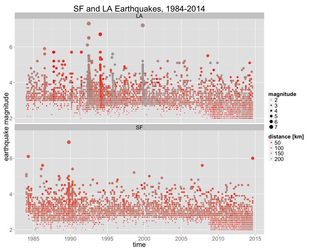
The major earthquakes that pop out in this plot are: Landers in 1992, Loma Prieta in 1989, and Northridge at the beginning of 1994. What is also interesting is the amount of aftershocks and related earthquakes for the major Los Angeles area earthquakes. Another interesting aspect of this plot is the increased detection efficiency of 2 to 2.5 magnitude earthquakes since 2009. Perhaps this is due to the Quake-Catcher Network (QCN)?
magnitude-frequency correlation
freq = as.data.frame(table(quakes[quakes$mag >= 2.0, c("area","mag")]))
freq = freq[order(freq$area),]
freq[freq$Freq == 0.0,] = NA # bins with zero counts cause log plot issues
png("SF-LA_magVfreq.png", width = 1000, height = 800)
magVfreq = ggplot(na.omit(freq), aes(mag, Freq)) +
           geom_point(aes(color = area), size = 4) +
           ggtitle("SF and LA Earthquakes, 1984-2014") +
           ylab("frequency [event count per 31 years]") +
           scale_y_log10(breaks = trans_breaks("log10", function(x) 10^x),
                         labels = trans_format("log10", math_format(10^.x))) +
           scale_x_discrete("magnitude", breaks = seq(2,7,1)) +
           geom_smooth(method = "loess", aes(group = 1), color = "black") +
           theme_grey(base_size = 12) +
           theme(text = element_text(size = 22))
print(magVfreq)
dev.off()
Output:
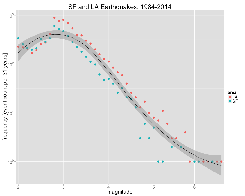
The correlation between magnitude and frequency for most of the Richter scale has a slope of about 10^1 events over one order of magnitude. Furthermore, as the magnitude increases, the spread of the data increases due to the insufficient amount of counts.
Code available on Github
The code for this post can be found under the exploration directory on github in my usgs repository: quakes.R
Many thanks to usgs.gov for providing easy access to their earthquake data.